March 16 – Airlines are in trouble and already there is talk of a $50 billion bailout. International travel is at a standstill, and companies are canceling routes at a furious pace. United Airlines is cutting its flying in half in April and May.
This of course brings back memories of the post 9/11 airline bailouts, where the government handed out $5 billion in cash to airlines and billions more in subsidized loans, insurance payments, and other benefits, although not all of the loans were used up. It should be noted that several airlines went into bankruptcy around that time, including United Airlines and US Airways.
The public health story line is, of course, the most crucial of all. But on the economic front, there are a number of important storylines to follow. This thread will be updated regularly.
Last updated: March 18th, 9:20 am.
Markets
Stock market. Down 30% so far, wiping $9 trillion off household balance sheets, including $1 trillion from 401ks.
Restaurants are struggling to survive. 5 major cities and several states have shuttered all restaurants. Foot traffic down 50% in many cities. Many restaurants going out of business and laying off workers.
Retail: many stores closed until end of March. As of yet, still paying workers. Most online stores staying open.
Monetary policy. Federal reserve cut interest rates to zero (the lower bound?) Quantitative easing is started.
Fiscal policy is still in its early stages. Trump proposes $850 billion stimulus, possibly including direct cash transfers. Small House Coronavirus bill still struggles to be passed.
Support for companies: airlines, hotels, and casinos asking for bailouts, but there is strong pushback.
Consumers
Overall spending, still little data. In Seattle, consumer spending with credit cards down 10%. Driven by hotels, movie theaters, restaurants. Spending on childcare, health care up big.
The one high point of consumer spending is the effect from consumers stocking up. Many shelves have been emptied, especially for toilet paper and cleaning supplies.
Data from China for January and February has just come in, and retail sales have dropped 20.5% year over year. This could be a preview of what is happening in the US, as many stores are now closing at a furious pace. USA Today has a roundup:
Apple is closing all stores outside of China until March 27. Employees will continue to be paid. The online store will be open.
Patagonia similarly is closing stores until March 27, and continuing to pay its workers. The online store will be closed as well.
Nike will be closing stores until March 27th.
lululemon, Abercrombie & Fitch, Lush, and Urban Outfitters are likewise closing their stories.
Columbia Sportswear, REI will likewise close. Roundup from Neil Saunders.
At least so far, the stores are continuing to pay employees. If stores remain closed past March 27th, this may change of course.
Malls, department stores, and other establishments are also cutting their hours, even if they are staying open.
On the flip side, sales at grocery stores and big box retailers have been boosted by people stocking up on supplies. Many shelves have been picked clean at Costco, and other stores are having to close early so the shelves can be restocked. There has been a “run” on every day staples such as toilet paper and hand sanitizer. It is unclear how long this panicked buying will last.
Continuing to wrap my head around the key economic story lines. Restaurant and bar employment is about 12.3 million, but as the virus spreads even further people aren’t going out to eat any more.
Data from Open Table shows that restaurant visits are down up to 50% in major cities such as Seattle, New York, and Boston.
This is big trouble for restaurants, who will close en masse if this keeps up. In Seattle, where the outbreak has hit the hardest, already 50 restaurants have closed.
To add to this, many states and cities are starting to show down or restrict the operation of restaurants and bars for the near term:
While some establishments can transition to take-out and delivery only, it is unclear the revenue drop from this switch and many will be forced to close.
In the short term it seems that many places will go out of business due to the fact they still have to pay leases, interest and debt, and sales tax. Quick relief for restaurant owners could come if the sales tax payment is deferred. Other potential relief for restaurant owners could come if lease payments are deferred.
Robert Shiller: “In 1933 when Roosevelt took office, he said there is “no plague of locusts” referring to the Depression. …There was no pandemic—no pandemic of insects or of viruses. But now there is. This is really different.”
WSJ: Companies have so far largely avoided layoffs. This may not last.
Bloomberg: Nice overview of the sectors that are more or less affected by the decline.
March 14
As the stock market plunged this past Monday, the denizens of Twitter awoke to find that all was not well with their stock portfolios. And as a researcher who studies the macroeconomic effects of the stock market, the results were interesting.
#My 401k and #blackmonday
Not surprisingly, the populi were concerned about their 401ks, which for many is the main source of retirement income, and #My 401k was trending.
From a few reactions it would seem that there may be a negative wealth effect.
Not everyone, however, was on board with this logic.
Facts don’t care about Haig-Simons income.
From a macroeconomic standpoint, while a falling stock market may be a sign that investors think a recession is coming, it can also itself be a potential cause of a recession. A major concern is that a falling stock market (a) could depress spending through a wealth effect (b) can influence spending through consumer confidence / a narrative of an economic collapse. And the numbers are not looking good. Although markets were up broadly on Friday, the Wilshire 5000, the broadest index of US stocks, was down 21% from its peak.
To get a back of the envelope estimate of this economic effect, before the crash Americans owned roughly $34 trillion in equities. A 21% decline is a hit to financial wealth of $7.2 trillion dollars. 401ks alone dropped in value by about $1 trillion. But how does this drop in stock market wealth effect the economy?
The best recent estimate of the effect of stock market wealth on spending is from Chodorow-Reich, Nenov, and Simsek, who find that people spend about 3.2 cents every year for every dollar of stock market wealth they own. A decline of the magnitude we’ve seen, if it persists, would then lead to a decline in consumer spending of $230 billion per year, or 1% of GDP.
Imagine a world in which the most pressing issue is to slash taxes for the rich and only the rich, costing the US government hundreds of billions of dollars and doing little to spur economic growth. Imagine a policy so unequal that even Mitt Romney has his doubts. Reader, I give you the capital gains tax cut.
Over the long run, the stock market has always gone up. This is the conclusion drawn from “Stocks for the Long Run”, Jeremy Siegel’s book about the long run returns of different asset classes. The real (inflation adjusted) returns on stocks from 1802-1871 was 7.0%. From 1872-2018, the real return was not much changed, 6.76%. During the post-war period, 1946-2018, returns were likewise similar at 6.82%. This remarkable stability of long-term real returns is a characteristic of mean reversion for equity prices.
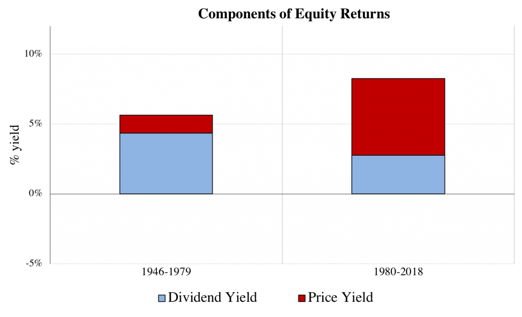
But within this stability of long-run returns, there have been important changes in the structure of returns over the past four decades. Stocks used to generated returns primarily through paying dividends, and to a lesser extent through price appreciation. From 1872-1979, 80% of stock returns were from dividends paid out, while 20% of returns came from price appreciation. But there was a reversal of this from 1980-2018: during this period 65% of returns came from price appreciation, and 35% from dividends.
Figure 1: Changing nature of equity returns. Data from Robert Shiller’s website.
Figure 1 decomposes total equity returns into its components: dividends and capital gains. We see that there has been a key shift over time away from dividends and towards capital gains.
Figure 2: Postwar bond slump.
There have also been shifts in the composition of bond returns over these two periods. Unfortunately for bond investors, over the long run the bond market has not always yielded high or constant returns. Figure 2 breaks down the inflation adjusted return on bonds in the postwar period. From 1946-1979, the average real bond return was negative, as inflation wiped away the value of coupons, while rising interest rates lead to capital losses on bonds. The story is quite different in the post-1980 period: low and stable inflation, combined with a fall in interest rates, led to adequate returns, although still lower than stocks. As Siegel notes, although stocks are riskier than bonds over short holding periods, once the holding period increases to between 15 and 20 years, the standard deviation of average annual returns become lower than the standard deviation of average bond returns. Over 30-year periods, equity risk falls to only two-thirds that of bonds.
While the cause of the shift in bond returns is straightforward enough, that of equity is more difficult. One important force that may be driving capital gains is the changing nature of corporate payouts. Instead of returning their earnings to shareholders through dividends, firms may be reinvesting their earnings, or using the cash to purchase their own shares — stock buybacks. Both uses of cash would boost share prices, relative to a dividend payout. There has been a lot of recent attention of the rise of corporatebuybacks in the US, and this has certainly played a role– more about that in a future post.
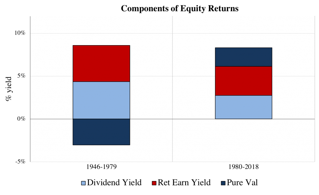
Figure 3: The Pure Capital Gain.
For now I want to examine to what extent capital gains are being driven by retained earnings. Under a Miller-Modigliani (1961) assumption that a dollar of post-tax earnings that is not paid out by the firm increases the value of the firm by a dollar, we can break down the amount by which price increases are being driven by retained earnings. The “price return” component of figure 1 is thus broken into two components in figure 3: a retained earnings yield, and a pure valuation increase. Pure valuations were negative for the first few decades of the post-war period, but since 1980 they have been positive and large.
The changing nature of returns has lead to a changing nature of income in the US, the increased importance of capital gains. More about this in future posts!
Robert Barro has a problem with GDP and national income. His complaint isn’t the usual modern one about the inability of GDP to properly measure the value of household production,gross national happiness,inequality, Ubers at 2:00 am, or the fresh aroma after a summer downpour. Instead it’s an older and crustier complaint, about the nature of investment and its relationship to income.
In a new NBER working paper, Double-Counting of Investment (see coverage at Marginal Revolution and VoxEU) Barro stacks several counts of charges against the current system of national accounts: (1) that “national income and product accounts double-count investment, which enters once when it occurs and again in present value when the cumulated capital leads to more rental income ” (2) that current concepts are conceptually baseless, as they are not grounded in individual optimization (3) that the national accounts do not properly account for welfare. According to Barro, “a necessary condition from an intertemporal perspective is that — at least conceptually– the present value of measured production and income should equal the present value of consumption.”
Claims about GDP
First question: does GDP double count investment? That depends on what GDP is trying to measure. The Bureau of Economic Analysis, the agency that compiles GDP, defines it as follows: “GDP measures the market value of the goods, services, and structures produced by the nation’s economy in a particular period. While GDP is used as an indicator of economic activity, it is not a measure of well-being (for example, it does not account for rates of poverty, crime, or literacy).” The goods in this case include not only consumption goods like food, but also investment goods like machines and factories. In trying to measure production which includes investment goods, there is naturally no double counting of investment goods if investment goods are indeed counted.
Barro of course knows this, but still he wants to use GDP as a foil for his new measures of economic welfare. So be it. But what of his new measures of national wellbeing?
Permanent income
Barro explores a different national accounting concept, one which corresponds more closely to the idea of Milton Friedman’s permanent income idea. The basic idea is that it is not just current period consumption that affects welfare, but the entire consumption or income over the lifetime. Since it is difficult to estimate future consumption, if we make assumptions about the structure of the economy, economic theory can provide a way to measure this future consumption. In particular, if the economy can be described by a representative agent framework in which the agent maximizes utility from consumption over an infinite horizon, this welfare is measurable.
The analysis starts from the intertemporal budget constraint from an infinitely lived representative agent:
(1)
where is capital, the wage, the labor supplied, is consumption, and is the return on capital rate, assumed to be constant. If we make the simplifying assumption that we are in a balanced growth path, with wages growing at rate and constant interest rates, we can then write
(2)
Correctly defined income can then be defined from the left hand side of the budget constraint, . This has the very nice property of falling directly out of an individual’s intertemporal budget constraint.
So under the assumptions that (1) the economy can be described in a representative agent framework (2) the economy is in the steady state (3) r, g, and K are able to be measured, we have a decent measure of an economy’s welfare.
The first problem arises when we think about how we would measure this equation. If we grant, for the moment, that we are in the steady state, there is still the problem to determine the long-run growth rate of the economy, as well as the return on capital. Given the work of Robert Gordon and others on the decline in productivity, it is not at all obvious what future productivity growth will be. The second problem is estimating the return on capital, as this requires an estimate of the risk premium on capital, another object with a large degree of uncertainty. The third problem is correctly estimating the capital stock, a very thorny task.
The problem becomes infinitely more intractable if we depart the steady state, a world in which undoubtably we are in. Then the nice properties of Barro’s framework go away, and we need to estimate the full path of wages, demographics, labor force participation, and interest rates. As far as I can tell, Barro doesn’t discuss at all how these will be estimated, and sticks instead to the measurement of steady state permanent income.
Another issue that may arise is if there is any departure from perfect competition in the economy. For example, if the pure profit share of the economy is , then then the budget constraint becomes
(3)
It would then be necessary to estimate the degree of pure profits in the economy, as well as GDP, in order to calculate permanent income.
Barro recognizes some of these difficulties, and proposes another way of estimating income. Instead of looking at the left hand side of equation (2), the second possibility is to calculate net product using the right hand side. In this case, gross investment is subtracted from gross product, and thus investment is 100% expensed and net product is exactly equal to consumption.
But true permanent income, as Barro conceptually defines it, is equal to the present discounted value of future consumption. In a steady state there are no problems, but outside of the steady state, the entire future path of consumption must be accounted for. And how should this be estimated?
Barro notes a related problem of the gross expensing of investing. Take Country A, with a GDP of $100 and a consumption of $10, and Country B with a GDP of $10 and a consumption of $10. Under Barro’s income concept, the two countries have the same income. Clearly there is a problem with this income concept, for it relies upon whether countries use their resources for current rather than future consumption. Barro realizes this problem: “the more general idea is that one would like a notion of current income that reveals, to the extent feasible, the possibilities for consumption in a full intertemporal sense.”
History of Economic Thought
Interestingly, Barro’s definition of income and production as pseudo consumption is quite close to that of Irving Fisher. There was a lively debate about this issue in the 1930s and 1940s between Fisher, Hicks, Kaldor and others (see the edited volume by Harcourt (1969)), which I believe sheds some light upon Barro’s claims. Fisher’s concept of income was as follows:
Real income … consists of those final physical events in the outer world which give us our inner enjoyments. This real income includes the shelter of a home, the music of a victrola or radio, the use of clothes, the eating of food, the reading of the newspaper, and all those other innumerable events by which we make the world about us contribute to our enjoyments.
Fisher thus defined income to be equal to consumption, quite similar to Barro. Fisher’s idea of ‘capital’ is quite similar to Barro’s permanent income type concept:
Capital, in the sense of capital value, is simply future income discounted or, in other words, capitalized. If Henry Ford receives $100,000,000 in dividends but reinvests all but $50,000, then his real income is only $50,000. This distinction between the real income, actually enjoyed, and the accretion or accrual of capital value, that is, the capitalization of future enjoyments… is in general vital.
The main criticism of Fisher from his contemporaries is that his particular concept of income is very different than the common one. As Erik Lindahl wrote (Lindahl 1969, same volume), “Irving Fisher’s analysis is carried out in masterly fashion, but all his attempts to demonstrate that his concept of income is the usual one and that it is the only logical one must be considered unsatisfactory. In neither popular nor scientific terminology are income and consumption equated; on the contrary, income is generally take to include saving (either positive or negative), and the crux of the matter is to decide just what this term saving may be taken to cover.”
Kaldor wrote of Fisher’s income concept, “Fisher tried to gain acceptance for a concept of income that is free of ambiguity and capable of measurement, but which plainly does not correspond with the sense of the everyday use of the term … Fisher’s approach has the virtue of yielding a simple and unambigulous result, but it does not accord with everyday notions on the subject; and in a sense, it only solves the problem by eliminating it.” Kaldor states a problem with the income-as-consumption concept that Barro also identifies: “Defining for the moment the 1net yield’ of all capital as consumption, this ‘net yield’ will depend not only on the quantities and the productivity of different kinds of resources in existence, but also on the dispositions of their owners as between using these resources for purposes of current consumption and using them for future consumption.”
Barro begins by approving quoting Kuznets (1941), the bible of national accounting, who at one point (p 46) muses that “since the final aim is to satisfy the wants of ultimate consumers, we might perhaps more properly center attention on ultimate consumption.” But Barro seems to have skipped over the entire rest of the book, as well as the rest of Kuznets’s oeuvre. He should have started on page 1, sentence 1: ”National income may be defined as the net value of all economic goods produced by the nation.”
Bibliography
Fisher, Irving. “Income and Capital.” In Readings in the Concept and Measurement of Income, edited by R.H. Parker and G.C. Harcourt, 33-53. Cambridge: Cambridge University Press, 1969.
Kuznets, Simon, Lillian Epstein, and Elizabeth Jenks. National income and its composition, 1919-1938. Vol. 1. New York: National Bureau of Economic Research, 1941.
Parker, Robert Henry, Geoffrey Colin Harcourt, and Geoffrey Whittington. Readings in the Concept and Measurement of Income. Cambridge University Press, 1969.
McCulla, S.H. and Smith, S., 2007. Measuring the Economy: A primer on GDP and the National Income and Product Accounts. Bureau of Economic Analysis, US Departament of Commerce.


 is capital,
  the wage,
  the labor supplied,
  is consumption, and
  is the return on capital rate, assumed to be constant. If we make the simplifying assumption that we are in a balanced growth path, with wages growing at rate
  and constant interest rates, we can then write
 . This has the very nice property of falling directly out of an individual’s intertemporal budget constraint.
  , then then the budget constraint becomes