I have some gripes on twitter about the Quantity Theory of Money. My main complaint is that everybody has their own private version of (i) which quantity theory they are talking about (ii) what definition of money they are using. So I thought I would lay out (a) all of the different versions that circulate (b) which ones I agree/disagree with.
A couple of recent pieces have revitalized the debate over whether money matters. The Washington Post has an interesting story about how Federal Reserve officials no longer care about the money supply:
But the current Fed chair, Jerome H. Powell, has dismissed claims that the Fed’s money-printing is fueling today’s price spiral, emphasizing instead the disruptions associated with reopening the economy. Like his most recent predecessors, dating to Alan Greenspan, Powell says that financial innovations mean there no longer is a link between the amount of money circulating in the economy and rising prices.
Krugman has likewise picked up on the comments from the Fed in his own blog post.
So what is the quantity theory of money. Jason Furman sets out the basic idea. The theory starts out from an accounting identity
M * V = P * T
M(oney) times V(elocity) equals P(rices) times T(ransactions). V(elocity) is supposed to roughly represent how many times a dollar changes hands in a given period. The “money” in this equation is usually taken to be a broad measure of money, such as M2, that includes checking account balances, some time deposits, as well as currency.
Now, transactions are very difficult to measure in the economy. Aside from buying and selling goods, transactions occur for financial assets, between banks, or when workers are paid — they are very difficult to get a handle on. And I don’t think anyone really even tries to make this work.
To make progress, we simplify and make the assumption that transactions are proportional to income (Y), giving the formula
M * V = P * Y
This is still (mostly) an accounting identity — but becomes a theory when we put additional structure on the equation. If we assume that velocity is roughly constant, we have
P = M*V / Y
Quantity Theory 1 (QT1): prices should grow at the roughly the rate of broad money minus the growth rate of output.
This is the classic statement of the quantity theory. For example, Wikipedia defines the quantity theory as “general price level of goods and services is directly proportional to the amount of money in circulation — the money supply.”
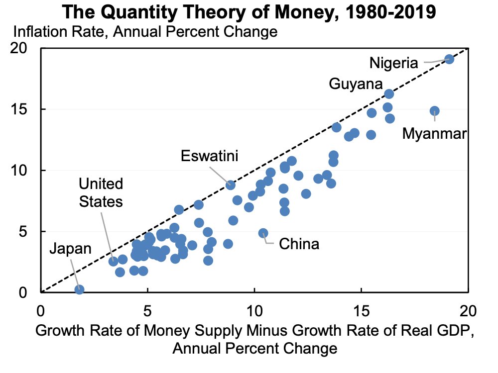
This is actually quite an interesting theory because it is a statement about a correlation of potentially endogenous variables. A theory that says there should be a correlation between variables! Okay, great. The beautiful thing about this theory is that we can go ahead and test it. In his twitter post, Furman gives the evidence that this tends to hold pretty well over long periods of time:

It turns out that even over relatively long periods of time this really doesn’t hold up once you throw out high inflation countries.
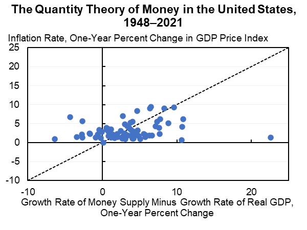
Over short periods, however, this doesn’t even come close to holding:

During the current pandemic there is been a dramatic drop in money velocity, again showing that the dramatic increase in M2 has not been matched with a commensurate rise in prices.

So my general view towards QT1 is that it holds in the long run but not in the short run.
Note, however, that this does not say anything about causality. In fact, I don’t that QT1 has any causal content as a theory. It does not state that money causes an increase in prices, or that nominal spending growth causes an increase in the money supply. It simply says that they should be correlated.
The reason why there is no causal content is because measures of broad money are an endogenous variable. The Federal Reserve does not directly control the level of M2 in the economy. In fact, under the Federal Reserve’s Ample Reserves regime, the Fed does not even strictly target the level of reserves in the economy.

Quantity Theory #2: the money multiplier version. An increase in base money translates to a given increase in broad money, and then to prices. This is the version that Art Laffer and others espoused during the Financial Crisis:
This is the worst version of the theory and is clearly contradicted by the data. First off, the “money multiplier” is not even close to constant and has seen wild fluctuations after the financial crisis. In a liquidity trap there should be little effect of an increase in base money on broad money aggregates.

Second, as discussed above, there isn’t much correlation between broad money and inflation at short time horizons. So both legs of this theory don’t work great.
Note that unlike QT1 this is a causal theory. So if it did hold (and it does not) we would at least
Quantity Theory #3: the “vaguely causal” version. An increase in broad money causes an increase in prices, but broad money is assumed to be exogenous.
This is often a version which crops up and is my least favorite because it is incomplete. If you are going make a causal statement of how broad money affects prices, you have to specify what is causing the change in broad money!
What is my takeaway from this tangle of thorns?
My baseline view of the world is similar to that of the Federal Reserve: monetary aggregates are endogenous. The money supply expands when the economy and credit expands, and contracts when the economy contracts. Given the evidence, I think the QT1 holds roughly in the long run but not in the short run, but this says nothing about the causal direction.
Now, I wouldn’t go as far to say that changes in the broad money supply are unimportant. In fact, a sharp contraction in broad money would be a very worrying sign of economic collapse, such as during the Great Depression.
But I would not use the MV = PY equation to understand the current state of the economy.